Technical white paper
From Erlang to Excel
Contact-centre queueing theory from beginner to expert — and how to rebuild every formula in a spreadsheet you control.
A ccPlanning technical white paper
Download the paper & the working workbook
The full paper as a PDF, plus a live Excel companion with every Erlang B/C/A formula already built — change the inputs and watch it recalculate.
Download the white paper (PDF) Download the Excel workbookWho this is for
If you have ever typed a call volume into an online Erlang calculator and trusted the number it gave back, this is for you. The goal is to take you from that black box to a place where you understand exactly what the calculation does, why it does it, and how to reproduce every figure yourself. It is written to be read in order: the early sections assume nothing beyond arithmetic and a working knowledge of a contact centre; by the end we derive abandonment from a birth–death Markov chain and discuss where the classical formulae stop being trustworthy.
The man behind the formulae
The mathematics in this paper carries one man’s name. Agner Krarup Erlang (1878–1929) was a Danish mathematician who graduated from the University of Copenhagen in 1901 with a sweep of subjects — mathematics, physics, astronomy and chemistry — then spent the better part of a decade as a schoolteacher, pursuing probability theory privately in his spare time. The decisive turn came in 1908, when he joined the Copenhagen Telephone Company as a scientific collaborator and head of its newly formed laboratory. For the first time a serious working mathematician was sitting inside a real, expensive operational problem.
That problem was provisioning. A telephone exchange needs circuits, and circuits cost money: too few and callers meet the engaged tone, too many and capital sits idle. Erlang reframed it as probability rather than guesswork. His 1909 paper, “The Theory of Probabilities and Telephone Conversations”, used real data from the Copenhagen exchange to show that calls arrive at random, following a Poisson distribution — the very assumption we lean on below. His 1917 paper then gave the loss and waiting-time formulae we still call Erlang B and Erlang C. From one practical need, he founded the disciplines of teletraffic engineering and queueing theory.
A century later, the same equations size far more than telephone trunks: contact-centre agents, computing clusters, checkout lanes, hospital beds — anywhere finite capacity meets random demand and service must be balanced against cost. The international unit of traffic load, the erlang, was named in his honour in 1946. So when you calculate the staffing for “80% answered in 20 seconds”, you are reaching for a tool a modest Danish engineer built to stop Copenhagen’s switchboards from jamming — and that is precisely why it still matters today.
The shape of the problem
Staffing a contact centre is a queueing problem. Work arrives at random; a finite number of agents handle it; if everyone is busy, the next contact waits. We want one thing above all: how many agents do we need so that a defined proportion of contacts is answered within a defined time — the service level, conventionally “80% in 20 seconds”.
What makes this hard is randomness. If 250 calls arrived exactly evenly and each took exactly 240 seconds, you could solve it with one division. They do not: calls cluster, handle times vary. That variability is what creates queues — and queueing theory is the mathematics of putting a number on it. The classical answer is three formulae from A. K. Erlang: Erlang B (a busy system blocks arrivals), Erlang C (they queue), and Erlang A (waiting callers abandon).
Offered load: the number everything hangs on
Before any service-level calculation we need the workload in a single unit: the Erlang. One Erlang is one continuous hour of work per hour of clock time — the average number of contacts in progress at once if there were no queueing.
All in the same units. In seconds, for the running example:
That is the floor on staffing: you can never meet demand with fewer than 33.33 agents, and because agents are whole people who need slack to stop queues exploding, you always need meaningfully more. How many more is what Erlang C tells us.
B13:  =B6*60          (interval length in seconds)
B14:  =B5*B7/B13      (offered load A, in Erlangs)
The assumptions behind the maths
Erlang’s formulae are exact — but only for a specific idealised system. Being honest about it is what separates a practitioner from a calculator operator. The models assume Poisson arrivals (random and independent; variance equals mean), exponential handle times (memoryless; real ones are closer to lognormal), a single homogeneous pool (every agent can take every contact), and statistical equilibrium (the queue settles within the interval). None is perfectly true; knowing where each bites lets you decide when Erlang is good enough and when to simulate.
Erlang B: blocking, and the recursion that tames it
Erlang B gives the fraction of arrivals that find every server busy in a system with no queue. We need it because Erlang C is most stably computed from it. The textbook form uses An over a factorial — both overflow a spreadsheet quickly. The fix is a recursion that never forms those big numbers:
Each step uses only the previous value. It is stable for any n you will meet. Sanity checks: B(1,1) = 0.5 and B(2,2) = 0.4.
A21:  =A20+1
B21:  =$B$14*B20/(A21+$B$14*B20)     (seed A20=0, B20=1; copy down)
Erlang C: the queueing workhorse
Erlang C is the model behind almost every staffing calculator. Same Poisson/exponential world, but with an unlimited queue and infinitely patient callers. The central quantity is the probability an arrival must wait:
Valid only when n > A; otherwise the system is unstable and the probability of waiting is effectively 1. From it we get the service level — an arrival either doesn’t wait, or waits in a queue draining at the spare capacity (n − A):
And two more outputs fall straight out:
Occupancy is the quiet constraint: a roster that hits service level at 95% occupancy burns agents out. Most centres cap planned occupancy near 85%.
Worked example
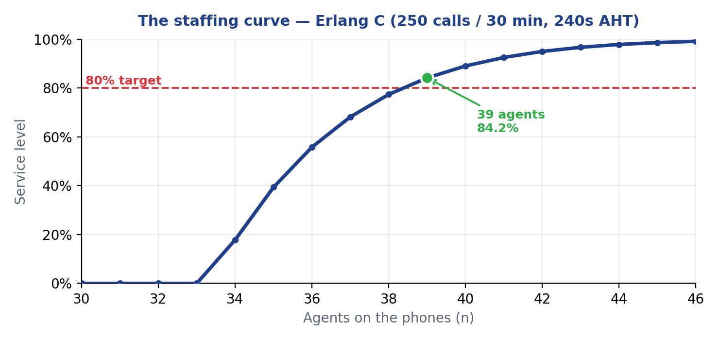
For A = 33.33 and a target of 80% in 20 seconds, watch how violently service level swings near the answer — the “power of one” every real-time analyst knows:
| Agents n | Erlang B | Erlang C | Service level | ASA (s) | Occupancy |
|---|---|---|---|---|---|
| 37 | 0.0700 | 0.4318 | 68.2% | 28.3 | 90.1% |
| 38 | 0.0579 | 0.3334 | 77.4% | 17.2 | 87.7% |
| 39 | 0.0471 | 0.2540 | 84.2% | 10.8 | 85.5% |
| 40 | 0.0378 | 0.1907 | 89.1% | 6.9 | 83.3% |
The smallest staffing meeting 80% in 20 seconds is 39 agents (84.2% SL, 10.8s ASA, 85.5% occupancy). Thirty-eight reach only 77.4% — one person is six points of service level.
C21:  =IF(A21<=$B$14,1,A21*B21/(A21-$B$14+$B$14*B21))      Erlang C
E21:  =IF(A21<=$B$14,0,1-C21*EXP(-(A21-$B$14)*$B$9/$B$7))   service level
F21:  =IF(A21<=$B$14,"",C21*$B$7/(A21-$B$14))              ASA
G21:  =IF(A21=0,0,$B$14/A21)                               occupancy
I21:  =IF(AND(E21>=$B$8,G21<=$B$10),A21,"")                 qualifying n
Agents required:  =MIN(I20:I100)
Prefer to skip the build? The same maths runs live in the free Erlang C and Erlang A calculators.
Erlang A: adding human patience
Erlang C’s biggest fiction is infinite patience. Real callers abandon — which both relieves the queue and represents lost service. Erlang A (the Palm / M/M/n+M model) adds a patience parameter. We model the system as a birth–death process: the state is the number of contacts in the system; arrivals push it up, completions and abandonments pull it down. Three rates govern it: arrival rate λ = contacts/interval, service rate μ = 1/AHT, and abandonment rate per waiting caller θ = 1/patience.
We build the relative weight of each state from the one below it — up to n only agents clear work; beyond n, waiting callers also abandon at rate θ:
Normalise (divide by the sum) to get probabilities p(k), then:
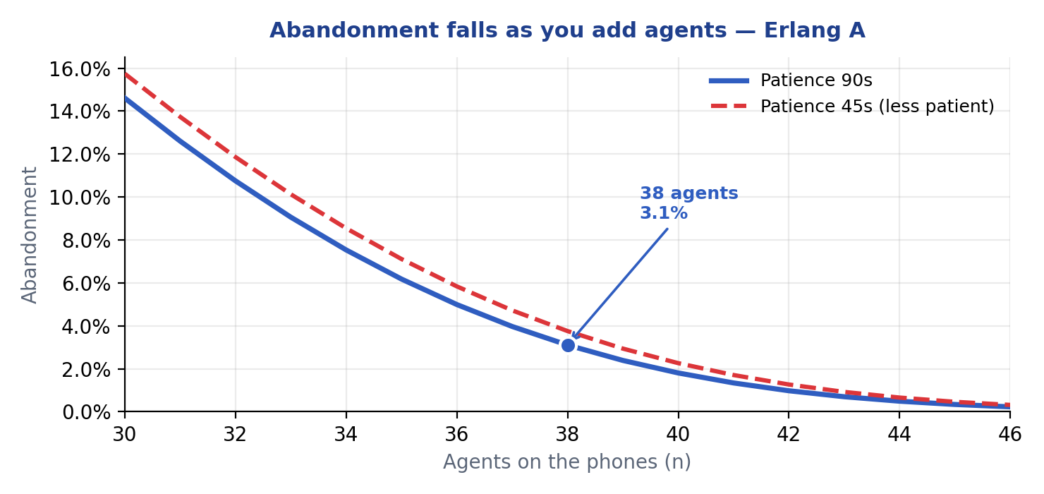
For the running example at 38 agents and 90-second patience: about 3.1% abandonment and an 18.6% chance of waiting — a more honest picture than Erlang C, which by construction can say nothing about abandonment at all.
B13:=B5/B7 (λ)   B14:=1/B6 (μ)   B15:=1/B8 (θ)
E22:  =IF(D22<=$B$9, E21*$B$12/D22, E21*$B$13/($B$9*$B$14+(D22-$B$9)*$B$15))
F22:  =E22/$B$16                                       p(k)
Abandon%: =B15*SUM(Gcol)/B13     P(wait): =SUMIF(Dcol,">="&B9,Fcol)
Erlang X: abandonment, blocking and redials
Erlang A added patience. Erlang X goes one step further and folds three real-world behaviours into a single model — the most realistic of the classical (non-simulation) formulae, and the default in several modern WFM tools. It was assembled in the 1990s by the Dutch mathematician Ger Koole, combining three properties earlier models handled only in isolation:
- Abandonment — callers leave when patience runs out (the Erlang A behaviour, first brought into queueing theory by Conny Palm in the 1960s).
- Blocking — a finite number of lines or a maximum queue size, beyond which new callers get a busy tone or are diverted (the Erlang B behaviour).
- Redials (retrials) — the genuinely new part: a fraction of callers who abandon, or hit a busy line, simply call back, adding to the load.
The redial property is what makes Erlang X more realistic and harder to compute, because it’s circular: abandoned and blocked calls generate redials, redials add to the load, more load means more abandonment and blocking, which generates more redials. There’s no neat closed form — it’s solved by fixed-point iteration: start from the base load, compute abandonment and blocking, add the redials back in, and repeat until the numbers settle.
Why it matters: Erlang C assumes everyone waits forever, which over-staffs an impatient queue — the “restaurant table effect” (book 50 tables for 70 couples and Erlang C waits all night, while in reality some leave and a few drift back). Erlang X captures that attrition and the persistent redials, so it sizes an impatient, line-limited operation more accurately — usually fewer agents than Erlang C, though barely different if your callers are patient. Reach for it when waits regularly creep above ~90 seconds, abandonment is non-trivial, lines are capped, or you want to see the redial load a busy signal creates.
In Excel: this is the one model you can’t lay down as a straight column — the redial loop is a circular reference. You have to enable iterative calculation (File → Options → Formulas, or Tools → Options → Calc in LibreOffice) so Excel re-feeds the redials into the load until it settles. The companion workbook does exactly that: its Erlang X sheet is built live, with iterative calculation switched on, so you can change patience, lines and the redial rate and watch blocking and abandonment move. You can also try it in the Erlang X calculator.
Where the formulae break
Reproducing the maths is one kind of mastery; knowing when not to trust it is the deeper one. Every assumption is a fault line:
- Non-Poisson arrivals. A marketing email or an outage makes arrivals burstier than Poisson, and real service level is then worse than Erlang C predicts.
- Handle-time distribution. Real handle times are lognormal, not exponential. It matters little for service-level sizing, more for wait-time variance and abandonment.
- The interval boundary. A sharp intraday ramp never reaches equilibrium; queues spill across 30-minute boundaries, so a per-interval Erlang sum understates busy-period pain.
- Multi-skill routing. The biggest limit: once agents share skills and contacts are routed between them, there is no closed-form Erlang. Pooled, cross-skilled operations beat the sum of their silos — the pooling gain — and only simulation captures it.
A discrete-event simulation drops all four assumptions — any arrival pattern, any handle-time distribution, a full skill matrix, continuous time, and patience — at the cost of returning a distribution rather than one exact figure. The practical rule: Erlang C for single-skill sizing, Erlang A when abandonment is material, and simulation for multi-skill, blended or strongly non-stationary work.
Which model, when
| Situation | Use | Why |
|---|---|---|
| Single queue, patient callers, SL target | Erlang C | The standard; fast and good enough |
| Single queue, callers abandon | Erlang A | Captures abandonment and queue relief |
| Abandonment + redials + capped lines | Erlang X | Adds redials and blocking on top of Erlang A |
| No-queue / trunk sizing | Erlang B | Blocking, not waiting |
| Multi-skill or blended routing | Simulation | No closed form exists |
| Very bursty or scheduled arrivals | Simulation | Poisson assumption fails |
| Long-range FTE / capacity | Workload + occupancy | Interval Erlang rolled up |
Build the spreadsheet once, validate it against the checks in the paper, and you will never have to take a black-box calculator’s word again.